PS Map¶

psmap() quantifies the 3d data/model agreement by computing the PS at each spatial bin in the ROI according to the algorithm described in Bruel P. (2021), A&A, 656, A81. (doi:10.1051/0004-6361/202141553). For each spatial bin, the algorithm first computes the data and model count spectra integrated over an energy dependent region (following the PSF energy dependence) and then computes the p-value that the data count spectrum is compatible with the model count spectrum (using the likelihood statistics). The absolute value of PS is -log10(p-value) and its sign corresponds to the sign of the sum over the spectrum of the residuals in sigma. The algorithm also provides a PS map in sigma units.

Caveat: the algorithm is currently not able to run in the context of a joint analysis with several event types.

Examples¶

In order to run psmap, the user must first compute the source model map using the write_model_map' function specifying the name of the model with the parameter ``model_name`(). The psmap() will then be called with the same model_name.

# Write the source model map (after performing the fit)
gta.write_model_map(model_name="model01")

# Generate the PS map
psmap = gta.psmap(model_name='model01', make_plots=True)

Configuration¶

The default configuration of the method is controlled with the psmap section of the configuration file. The default configuration can be overriden by passing the option as a kwargs argument to the method.

If the analysis uses likelihood weights, the user can specify the likelihood weight file with the argument wmap.

The user can set the parameters defining the energy dependent region used in the count spectrum integration step. The integration radius is defined by the function sqrt(psfpar0^2*pow(E/psfpar1,-2*psfpar2) + psfpar3^2), with E in MeV. The default parameters (``psfpar0``=4.0,``psfpar1``=100,``psfpar2``=0.9,``psfpar3``=0.1) are optimized to look for point-source like deviations. When looking for extended deviations (~1deg scale), it is recommended to use (``psfpar0``=5.0,``psfpar1``=100,``psfpar2``=0.8,``psfpar3``=1.0).

The user can set the energy range with the arguments emin and emax. Depending on the energy binning, it can be optimal to rebin the count spectra thanks to the argument rebin. For an analysis with 10 bins per decade, it is recommended to set rebin to 3.

*psmap* Options¶
Option	Default	Description
`chatter`	1	output verbosity
`emax`	1000000000.0	maximum energy/MeV
`emin`	1.0	minimum energy/MeV
`fixedradius`	-1.0	Fixed radius
`ipix`	-1	number of pixel i axis
`jpix`	-1	number of pixel j axis
`make_plots`	False	Generate diagnostic plots.
`maxpoissoncount`	100	Maximum number of poisson counts
`model_name`	None	Model name
`nbinpdf`	50	Number of bin of the PSF
`outfile`	psmap.fits	outfile name
`prob_epsilon`	1e-07	precision parameter
`psfpar0`	4.0	PSF parameter 0
`psfpar1`	100	PSF parameter 1
`psfpar2`	0.9	PSF parameter 2
`psfpar3`	0.1	PSF parameter 3
`rebin`	1	Rebin
`scaleaxis`	20	SCale axis
`wmap`		weight 3d map
`write_fits`	True	Write the output to a FITS file.

Output¶

psmap() returns a dictionary containing the following variables:

Key	Type	Description
psmax	float	maximum of the ps map
coordname1	str	Name of the coordinate of the ps maximum
coordname2	str	Name of the coordinaste of the ps maximum
coordx	float	Value of the X coordinate of the ps maximum
coordy	float	Value of the Y coordinate of the ps maximum
ipix	int	Value of the i pixel of the of the ps maximum
jpix	int	Value of the j pixel of the of the ps maximum
wcs2d	WCS Keywords	WCS of the ps map
psmap	np.array	PSMAP
psmapsigma	np.array	PSMAP in sigma units
name	str	NAmke of the model
ps_map	`Map`	WcsNDMap PSMAP
pssigma_map	`Map`	WcsNDMap PSMAP in sigma units
config	dict	Dictionary of the input configuration
file	str	Name of the output file
file_name	str	Full path of the output file

The write_fits option can used to write the output to a FITS or numpy file. The value of the maximum of the PS map can be retrieved from the output dictionary:

print('PS maximum value=%.2f, at %s=%.2f, %s=%.2f' %(psmap['psmax'],
                                                  psmap['coordname1'],float(psmap['coordx']),
                                                  psmap['coordname2'],float(psmap['coordy'])))

PS maximum value=3.85, at GLON-AIT=86.75, GLAT-AIT=38.62

Diagnostic plots can be generated by setting make_plots=True or by passing the output dictionary to make_psmap_plots:

psmap = gta.psmap(model_name='model01', make_plots=True)
//equivalent to:
gta.plotter.make_tsmap_plots(psmap, roi=gta.roi)

This will generate the following plots:

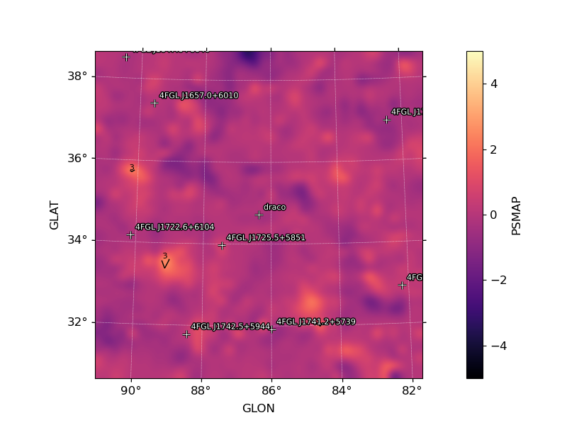
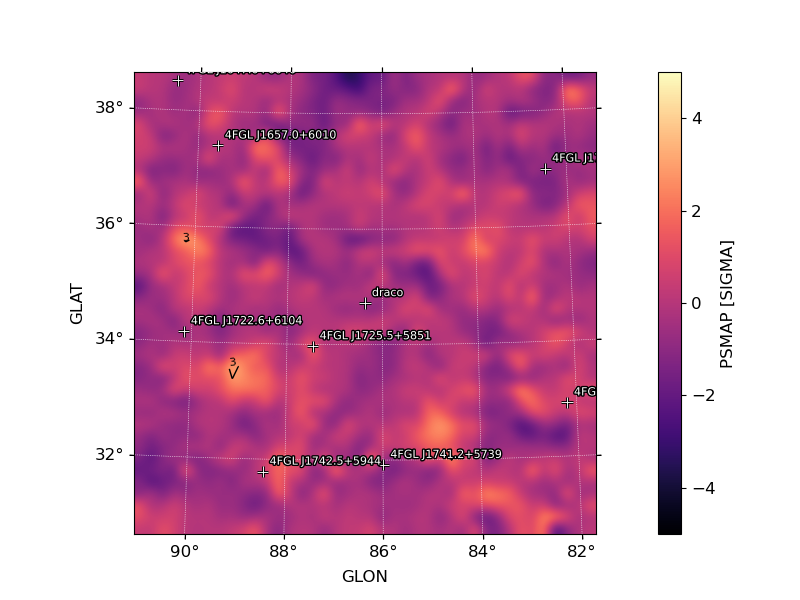
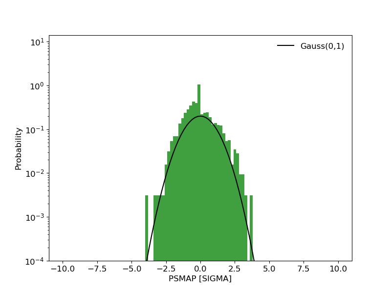
image_psmap : Map of PS values. The color map is truncated at 5 sigma with isocontours at 3,4,5 PS intervals indicating values above this threshold.
image_pssigma : Map of PS values converted in sigma. The color map is truncated at 5 sigma with isocontours at 3,4,5 PS intervals indicating values above this threshold.
image_ps_hist : Histogram of PS values for all points in the map. Overplotted is the reference distribution for a gaussian with mean 0 and sigma=1.

PS Map	Sigma (PS) Map	PS Histogram

Reference/API¶

GTAnalysis.psmap(prefix='', **kwargs)

Generate a spatial PS map for evaluate the data/model comparison The PS map will have the same geometry as the ROI. The output of this method is a dictionary containing Map objects with the PS amplitude and sigma equivalent. By default this method will also save maps to FITS files and render them as image files. psmap requirtes a model map to be compute, therefore the user must run gta.write_model_map(model_name=”model01”) before running psmap = gta.psmap(model_name=’model01’)

Parameters:

prefix (str) – Optional string that will be prepended to all output files.
kwargs (Any) – these will override the psmap configuration file
{options} –

Returns:

psmap – A dictionary containing the Map objects for PS and source amplitude.

Return type:

dict